MPI II: Domain decomposition

Today’s assignment

Domain decomposition

Domain decomposition is a frequently used method to parallelize programs that work with data on a (typically spatial) domain. In a nutshell, the idea is to decompose the global domain into a number of local subdomains, and then distribute those subdomains onto available processors – that’s actually similar to what OpenMP ended up doing for us when parallelizing the test_average example, though OpenMP only distributed the work, not the actual data (which was simply shared)

We could revisit the “average from node-centered to cell-centered” example, and get it to work in parallel with MPI. However, that example is a rather artificial, and also bit atypical in that the algorithm has asymmetry which unnecessarily makes it a bit confusing. A similar but much more common task is having to calculate derivatives, like in fact you may have already done in the KdV project.

I’ve added a new example as test_derivative.cxx for us to learn about ghost cells (a.k.a. guard cells, a.k.a. halos). It calculates the 2nd order approximation to the derivative of the sine function.

I’ll show some of the steps involved in class, but you can look at them in more depth and at your own pace in the assignment repo. This example is meant to to achieve two objectives:

• Demonstrate problems / special cases at boundaries, and how to use ghost cells to help with these.

• Learn how domain decomposition is implemented in an MPI parallelized code.

Boundaries

You can follow the history by looking at the commits in your assignment repo.

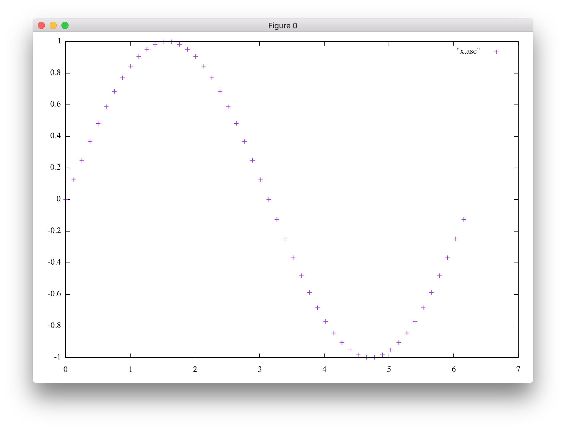
• The first step was to discretize the sine function and write it to a file, so that I could plot it. xtensor made this pretty simple. I chose to use the built-in support for CSV output, which means plotting the data in gnuplot needs one extra step:

kai@kais-mbp ~/class/iam851/iam851/build $ gnuplot

G N U P L O T
Version 5.2 patchlevel 7    last modified 2019-05-29

Copyright (C) 1986-1993, 1998, 2004, 2007-2018
Thomas Williams, Colin Kelley and many others

gnuplot home:     http://www.gnuplot.info
faq, bugs, etc:   type "help FAQ"
immediate help:   type "help"  (plot window: hit 'h')

Terminal type is now 'aqua'
gnuplot> set datafile separator ','
gnuplot> plot "f.csv" w lp

If you’re into not quite as antiquated tools, I also added a Python notebook that does the same thing in Pandas/matplotlib notebook.

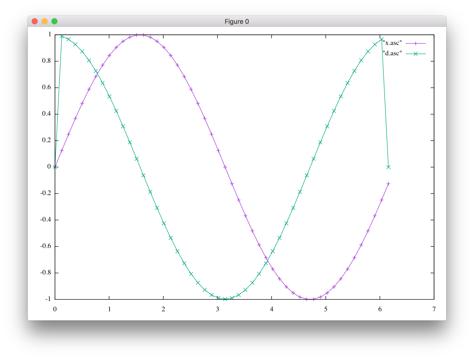
• The next step was to actually calculate the derivative, which should be the cosine, and that mostly works:

gnuplot> plot "f.csv" w lp, "f.csv" u 1:3 w lp

Or see the notebook.

• As you can see, the very first and last point of the derivative wasn’t right – and that’s because I hadn’t calculated it at all, since using my usual formula, I would have accessed the array out of bounds (e.g., on the left, I would have accessed f(-1)).

  xtensor has a special way to deal with periodic functions, but a more general way is to special case the two boundary points, again using that my function is periodic.

• It would be much more convenient, though, if I could just use the same calculation everywhere, including at the boundary. Well, I would be able to do that if my x array was extended one point on each side, ie. instead of having f(0), f(1), ... f(N-1), I’d like to have f(-1), f(0), ..., f(N-1), f(N). While this can be done in plain C/C++ with some hackery (normal arrays always start at 0), it’s not something that can easily be done on top of xtensor, which always uses 0-based indexing as well.

• So while I kinda like to think about having my 16-element array f indexed from 0..15 be extended by one point on each side to -1..16, I can’t do that, and instead will have to use 0..17 for the extended array f_g that now includes a ghost cell on each side. I made this (maybe) a bit less awkward by defining a constant G = 1 (as in ghost point) that I use to shift the indices.

  Having done that, I can now use the same formula to calculate the derivative everywhere.

  

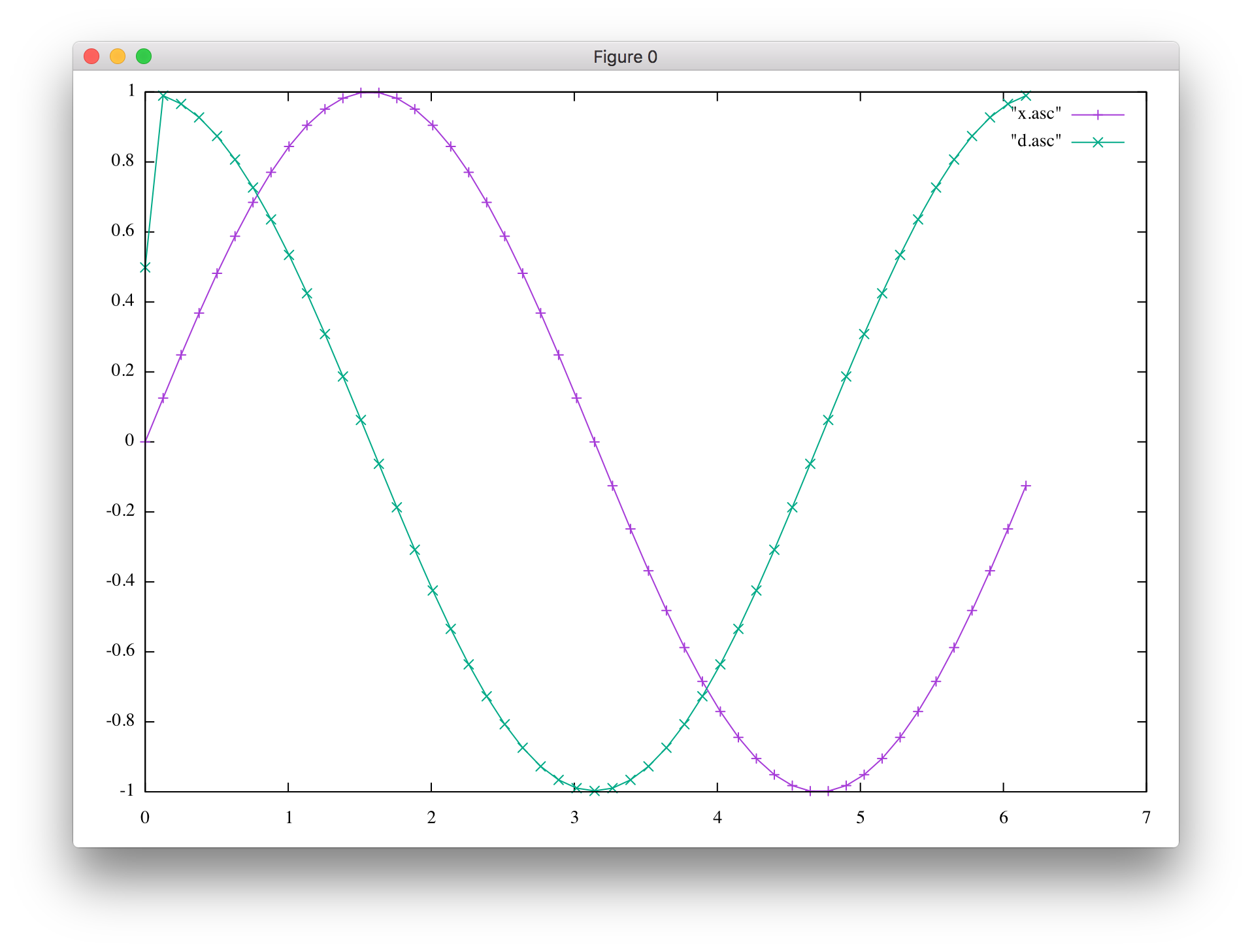
• However, the result still isn’t quite right, and that’s because while I’m using my extended f_g array now, I didn’t actually set any values into those additional cells, so they’re left at 0. After setting the ghost points to the correct values, it’s all good now.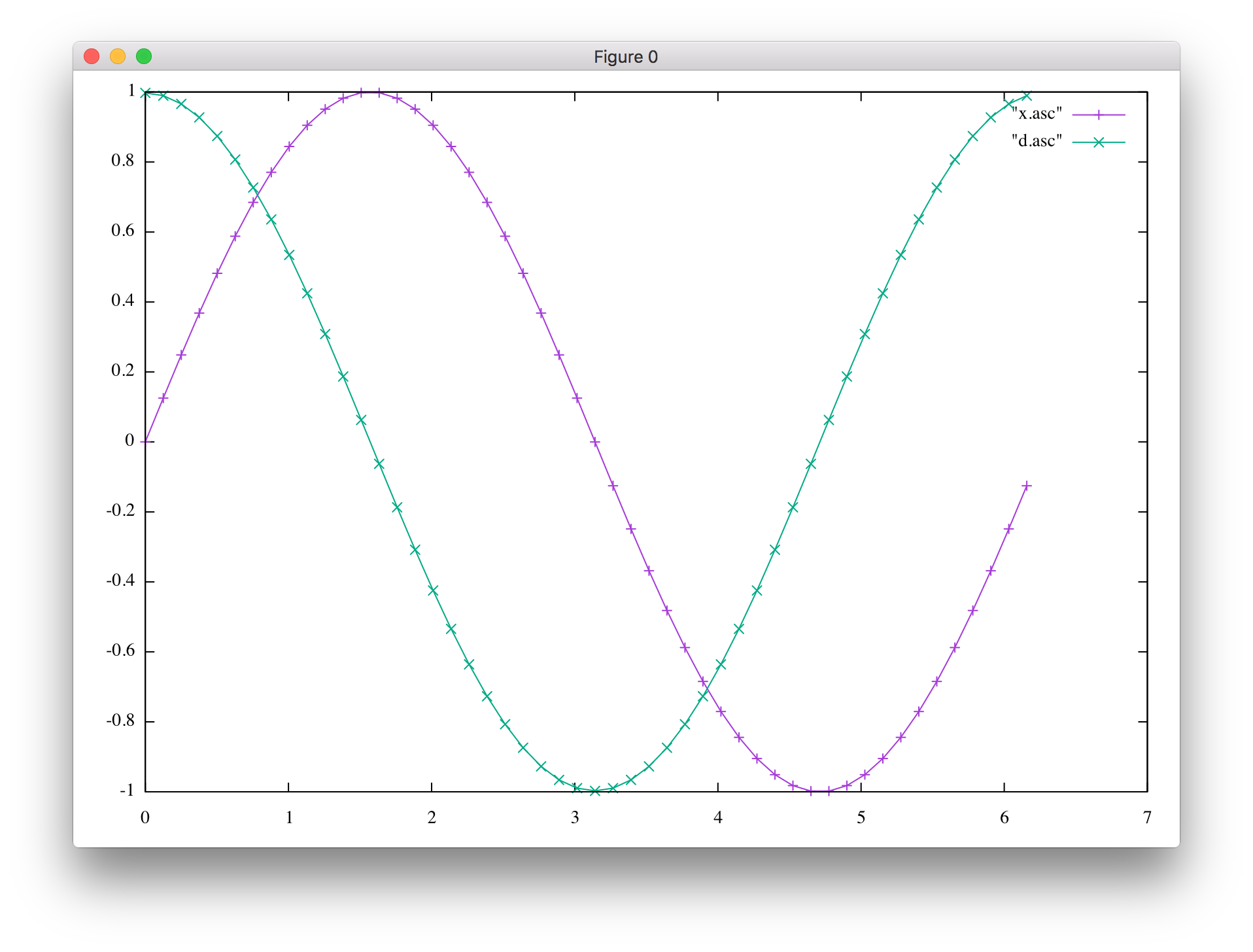

  

  Notebook.

• I couldn’t resist showing having xtensor allows one to do the same calculation more easily by using slicing similar to what can be done in Python/numpy. But that still needs ghost points.

• Finally, I made a smaller change in how the grid itself is generated.

Domain decomposition

So now that we’ve learned how to use ghost points to handle the case where we want to calculate a value at / near the boundary which requires values that aren’t part of the “true” domain, this will come in handy as we divide our spatial domain into multiple subdomains, each to be handled by a different MPI process, as that creates new artificial boundaries where those subdomains begin and end.

I left parallelizing this example using domain decomposition as an exercise for you. Here is my recommendation on which steps to follow:

Your turn

• The first step is to just add the usual MPI boilerplate code. (init, finalize, probably will need rank and size, too).

• Now, split the the [0:32) points into two halves:[0:16) and [16:32) to be handled by the two MPI processes. You can make the assumption that the code will be run with two procs for now – but it’d be good to at least add an assert to check that.

• Split the domain (x) so that the two procs handle [ \(0:\pi\) ) and [ \(\pi:2\pi\) ), respectively. Make sure this works correctly, for example by printing x (std::cout << x << "\n";).

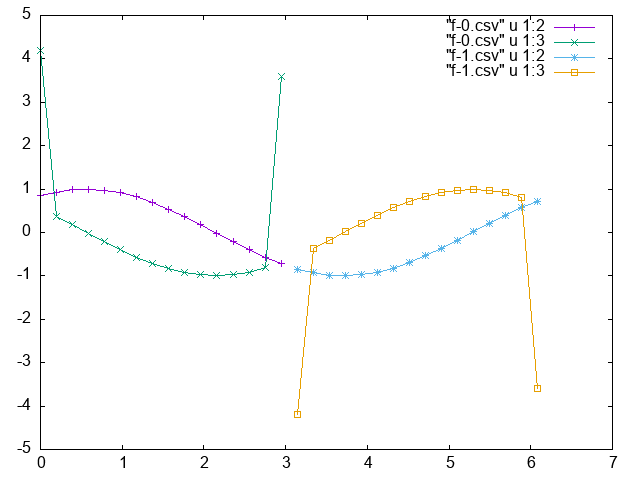
• The sine itself (f) should now also be split. In order to be able to plot things to make sure, you can’t have two procs write into the same file at the same time. So, create two output files, one per rank, e.g., f-0.csv and f-1.csv.

  This has the disadvantage that we need to plot data from multiple files to get all our data into the plot. On the other hand, it’s kinda helpful in understanding what data is on which proc for now.

• When looking at the actual derivative, hopefully, everything looks perfectly fine, except at the boundaries.

  

  [I phase-shifted my initial sine – it’s not crucial, but it does make for a better test. Why?]

• So here’s the main task: The ghost cells still need to be filled correctly, and that does involve sending messages from the proc that knows the actual value to the other proc that needs to put it into the ghostcells.

And once this works, it’s back to making sure that the code works more generally. In particular, don’t make it work for just N = 32 grid points, but things should still work if N is changed. It should also work when running on a different number of procs. You don’t have to be totally generic, you can impose reasonable constrains (e.g., total number of grid points must be divisible by the number of procs)

Homework

• As usual, complete the tasks given above, commit as you go and comment. Adding plots along the way will be helpful, too.